![]()
Results Plotting
This is a simple notebook displaying some of the results visualisation functionalities available in aeon.
This is in-progress, and does not contain detailed descriptions and documentation yet.
[1]:
import numpy as np

classifiers = ["Classifier 1", "Classifier 2", "Classifier 3", "Classifier 4"]
classifier_accuracies = [
    [0.8, 0.7, 0.6, 0.5],
    [0.7, 0.9, 0.4, 0.0],
    [0.8, 0.7, 0.6, 0.5],
    [0.7, 0.9, 0.4, 0.0],
    [0.7, 0.6, 0.5, 0.4],
]
regressor_preds = [0.8, 0.7, 0.6, 0.5]
regressor_targets = [0.9, 0.7, 0.4, 0.0]
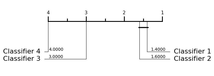
Critical Difference
[2]:
from aeon.visualisation import plot_critical_difference
[3]:
_ = plot_critical_difference(classifier_accuracies, classifiers)
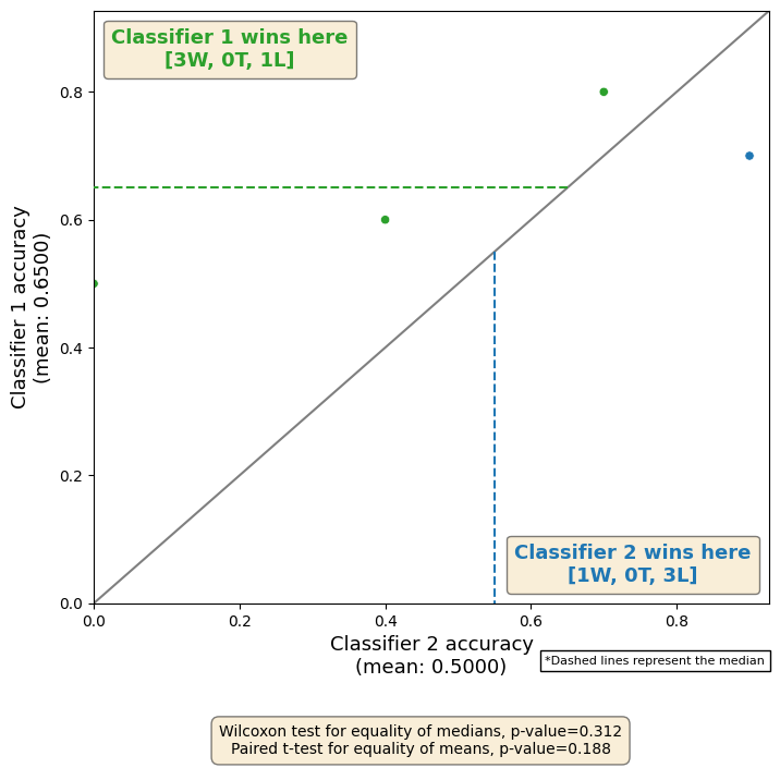
Scatter Diagrams
[4]:
from aeon.visualisation import (
    plot_pairwise_scatter,
    plot_scatter_predictions,
    plot_score_vs_time_scatter,
)
[5]:
_ = plot_pairwise_scatter(
    classifier_accuracies[0], classifier_accuracies[1], classifiers[0], classifiers[1]
)
[6]:
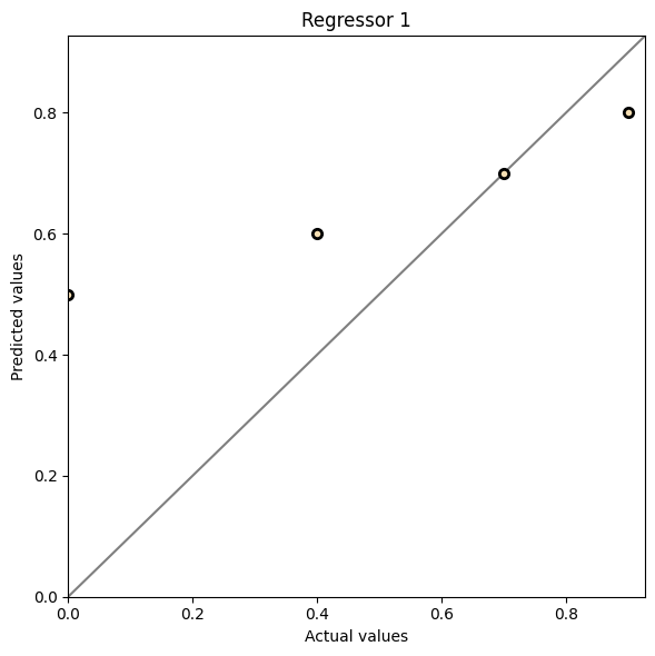
_ = plot_scatter_predictions(regressor_targets, regressor_preds, title="Regressor 1")
[7]:
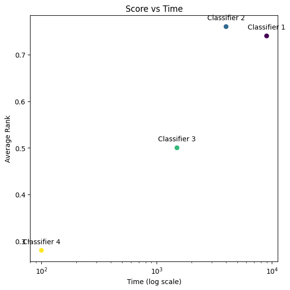
_ = plot_score_vs_time_scatter(
    np.mean(classifier_accuracies, axis=0),
    [9000, 4000, 1500, 100],
    names=classifiers,
    title="Score vs Time",
    log_time=True,
)
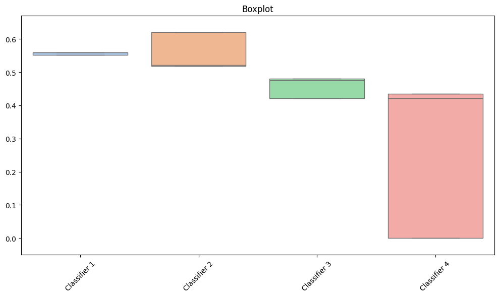
Box Plots
[8]:
from aeon.visualisation import plot_boxplot
[9]:
_ = plot_boxplot(
    classifier_accuracies,
    classifiers,
    relative=True,
    plot_type="boxplot",
    title="Boxplot",
)
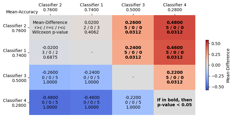
Multiple Comparison Matrix
A multiple comparison matrix is a heat map that shows the results of multiple pairwise comparisons between classifiers. It is highly configurable. You can save the figure to pdf or png, or even output the matrix as native latex code. A couple of examples follow
[2]:
import pandas as pd

df = pd.DataFrame(classifier_accuracies, columns=classifiers)
df.head()
[2]:
| Classifier 1 | Classifier 2 | Classifier 3 | Classifier 4 | |
|---|---|---|---|---|
| 0 | 0.8 | 0.7 | 0.6 | 0.5 |
| 1 | 0.7 | 0.9 | 0.4 | 0.0 |
| 2 | 0.8 | 0.7 | 0.6 | 0.5 |
| 3 | 0.7 | 0.9 | 0.4 | 0.0 |
| 4 | 0.7 | 0.6 | 0.5 | 0.4 |
[3]:
from aeon.visualisation import create_multi_comparison_matrix

create_multi_comparison_matrix(df, fig_size="8,4")
[3]:
<Figure size 640x480 with 0 Axes>
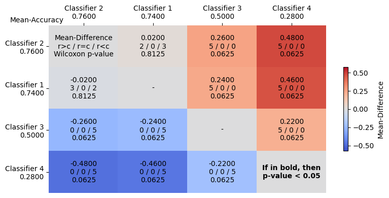
[4]:
from aeon.visualisation import create_multi_comparison_matrix

create_multi_comparison_matrix(
    df, fig_size="8,4", pvalue_test_params={"alternative": "two-sided"}
)
[4]:
<Figure size 640x480 with 0 Axes>
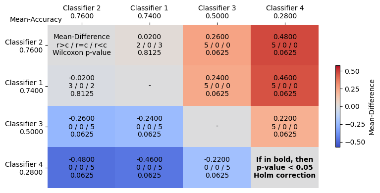
[5]:
from aeon.visualisation import create_multi_comparison_matrix

create_multi_comparison_matrix(
    df,
    fig_size="8,4",
    pvalue_test_params={"alternative": "two-sided"},
    pvalue_correction="holm",
)
[5]:
<Figure size 640x480 with 0 Axes>
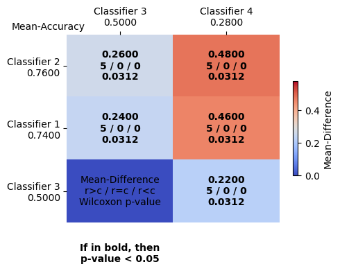
[24]:
from aeon.visualisation import create_multi_comparison_matrix

create_multi_comparison_matrix(
    df,
    fig_size="5,4",
    row_comparates=["Classifier 1", "Classifier 2", "Classifier 3"],
    col_comparates=["Classifier 3", "Classifier 4"],
)
[24]:
<Figure size 640x480 with 0 Axes>
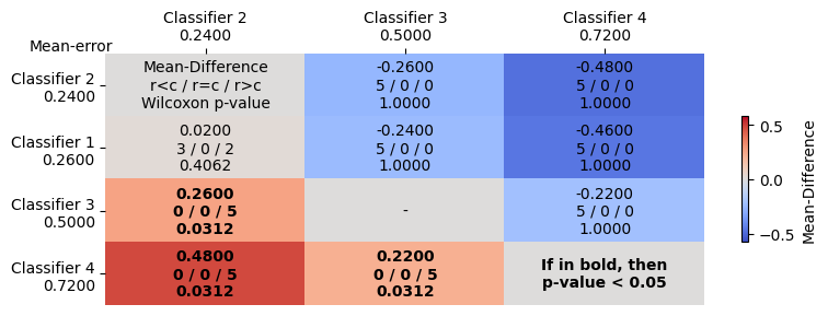
[17]:
errors = 1 - np.array(classifier_accuracies)
df2 = pd.DataFrame(errors, columns=classifiers)

create_multi_comparison_matrix(
    df_results=df2,
    excluded_col_comparates=["Classifier 1"],
    used_statistic="error",
    order_better="increasing",
    order_win_tie_loss="lower",
    fig_size="8,3",
    win_label="r<c",
    loss_label="r>c",
)
[17]:
<Figure size 640x480 with 0 Axes>
Generated using nbsphinx. The Jupyter notebook can be found here.