![]()
Analysis of the speedups provided by similarity search module
In this notebook, we will explore the gains in time and memory of the different methods we use in the similarity search module.
[1]:
import numpy as np
import pandas as pd
from matplotlib import pyplot as plt

from aeon.similarity_search._commons import (
    naive_squared_distance_profile,
    naive_squared_matrix_profile,
)
from aeon.similarity_search.distance_profiles.squared_distance_profile import (
    normalised_squared_distance_profile,
    squared_distance_profile,
)
from aeon.similarity_search.matrix_profiles import stomp_squared_matrix_profile
from aeon.utils.numba.general import sliding_mean_std_one_series

ggplot_styles = {
    "axes.edgecolor": "white",
    "axes.facecolor": "EBEBEB",
    "axes.grid": True,
    "axes.grid.which": "both",
    "axes.spines.left": False,
    "axes.spines.right": False,
    "axes.spines.top": False,
    "axes.spines.bottom": False,
    "grid.color": "white",
    "grid.linewidth": "1.2",
    "xtick.color": "555555",
    "xtick.major.bottom": True,
    "xtick.minor.bottom": False,
    "ytick.color": "555555",
    "ytick.major.left": True,
    "ytick.minor.left": False,
}

plt.rcParams.update(ggplot_styles)
Computing means and standard deviations for all subsequences
When we want to compute a normalised distance, given a time series X of size m and a query q of size l, we have to compute the mean and standard deviation for all subsequences of size l in X. One could do this task by doing the following:
[2]:
def rolling_window_stride_trick(X, window):
    """
    Use strides to generate rolling/sliding windows for a numpy array.

    Parameters
    ----------
    X : numpy.ndarray
        numpy array
    window : int
        Size of the rolling window

    Returns
    -------
    output : numpy.ndarray
        This will be a new view of the original input array.
    """
    a = np.asarray(X)
    shape = a.shape[:-1] + (a.shape[-1] - window + 1, window)
    strides = a.strides + (a.strides[-1],)
    return np.lib.stride_tricks.as_strided(a, shape=shape, strides=strides)


def get_means_stds(X, query_length):
    """Compute the means and standard deviations of rolling windows in a time series."""
    windows = rolling_window_stride_trick(X, query_length)
    return windows.mean(axis=-1), windows.std(axis=-1)


rng = np.random.default_rng(12)
size = 100
query_length = 10

# Create a random series with 1 feature and 'size' timesteps
X = rng.random((1, size))
means, stds = get_means_stds(X, query_length)
print(means.shape)
(1, 91)
One issue with this code is that it actually recompute a lot of information between the computation of mean and std of each windows. Suppose that the window we compute the mean for W_i = {x_i, ..., x_{i+(l-1)}, to do this, we sum all the elements and divide them by l. You then want to compute the mean for W_{i+1} = {x_{i+1}, ..., x_{i+1+(l-1)}, which shares most of its values with W_i expect for x_i and x_{i+1+(l-1).
The optimization here consists in keeping a rolling sum, we only compute the full sum of the l values for the first window W_0, then to obtain the sum for W_1, we remove x_0 and add x_{1+(l-1)} from the sum of W_0. We can also a rolling squared sum to compute the standard deviation.
The sliding_mean_std_one_series function implement the computation of the means and standard deviations using these two rolling sums. The last argument indicates the dilation to apply to the subsequence, which is not used here, hence the value of 1 in the code bellow.
[3]:
sizes = [500, 1000, 5000, 10000, 25000, 50000]
query_lengths = [50, 100, 250, 500]
times = pd.DataFrame(
    index=pd.MultiIndex(levels=[[], []], codes=[[], []], names=["size", "query_length"])
)
# A first run for numba compilations if needed
sliding_mean_std_one_series(rng.random((1, 50)), 10, 1)
for size in sizes:
    for query_length in query_lengths:
        X = rng.random((1, size))
        _times = %timeit -r 7 -n 10 -q -o get_means_stds(X, query_length)
        times.loc[(size, query_length), "full computation"] = _times.average
        _times = %timeit -r 7 -n 10 -q -o sliding_mean_std_one_series(X, query_length, 1)
        times.loc[(size, query_length), "sliding_computation"] = _times.average
[4]:
fig, ax = plt.subplots(ncols=len(query_lengths), figsize=(20, 5), dpi=200, sharey=True)
for j, (i, grp) in enumerate(times.groupby("query_length")):
    grp.droplevel(1).plot(label=i, ax=ax[j])
    ax[j].set_title(f"query length {i}")
    ax[j].set_yscale("log")
ax[0].set_ylabel("time in seconds")
plt.show()
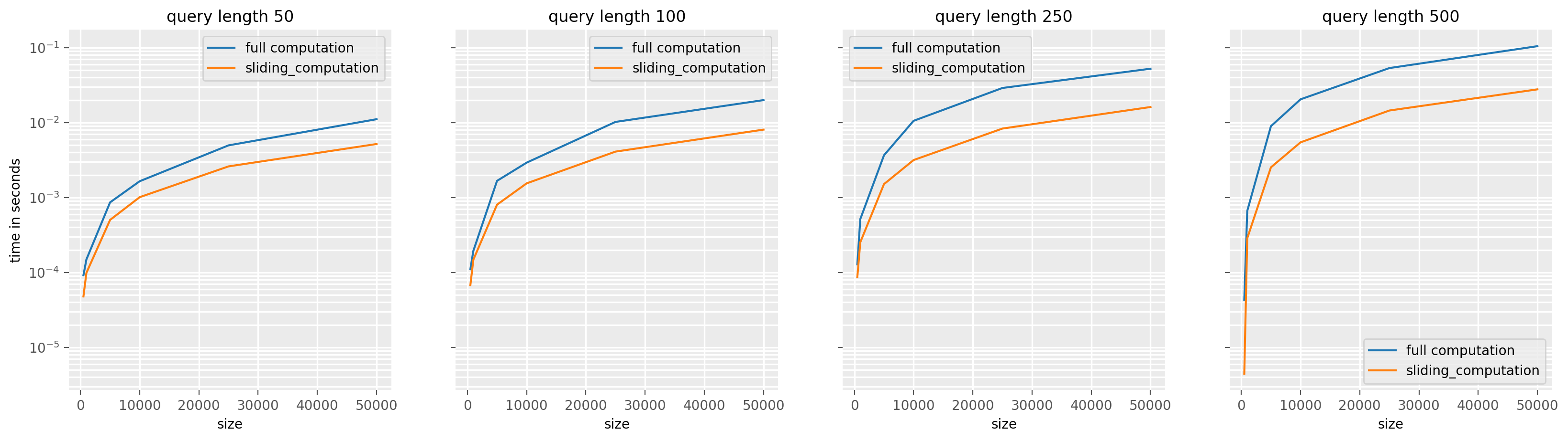
As you can see, the larger the size of q, the greater the speedups. This is because the larger the size of q, the more recomputation we avoid by using a sliding sum.
Computing the Euclidean distance with a dot product obtained from convolution
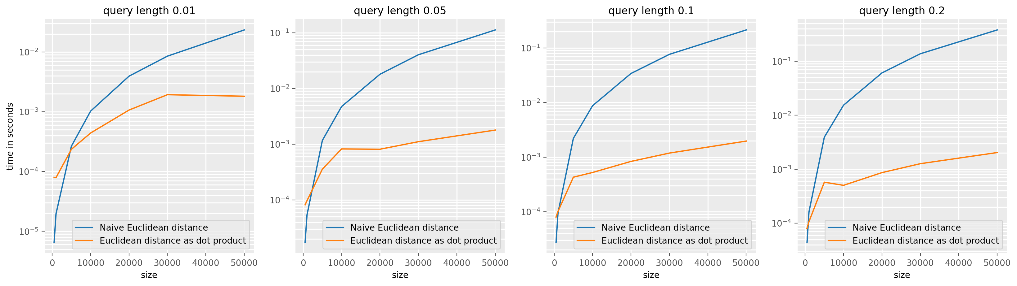
The standard way to compute the (squared) euclidean distance between a query Q = {q_1, ..., q_l} and a candidate subsequence W_i = {x_i, ..., x_{i+(l-1)} is to compute it as \(d(Q,W_i) = \sum_j^l (x_{i+j} - q_j)^2\).
We can also express this distance as \(d(Q,W_i) = Q^2 + W_i^2 - 2Q.W_i\), in our case, we can use the fact a cross corelation can be used to compute \(Q*X\) to obtain the dot products between \(Q\) and all \(W_i\). The timing difference become even more important for large input, when it becomes worth to use a fast Fourrier transform to compute the convolution in the frequency domain. See scipy.signal.convolve documentation for more information.
[5]:
sizes = [500, 1000, 5000, 10000, 20000, 30000, 50000]
query_lengths = [0.01, 0.05, 0.1, 0.2]
times = pd.DataFrame(
    index=pd.MultiIndex(levels=[[], []], codes=[[], []], names=["size", "query_length"])
)

for size in sizes:
    for _query_length in query_lengths:
        query_length = int(_query_length * size)
        X = rng.random((1, 1, size))
        q = rng.random((1, query_length))
        mask = np.ones((1, size - query_length + 1), dtype=bool)
        # Used for numba compilation before timings
        naive_squared_distance_profile(X, q, mask)
        _times = %timeit -r 3 -n 7 -q -o naive_squared_distance_profile(X, q, mask)
        times.loc[(size, _query_length), "Naive Euclidean distance"] = _times.average
        # Used for numba compilation before timings
        squared_distance_profile(X, q, mask)
        _times = %timeit -r 3 -n 7 -q -o squared_distance_profile(X, q, mask)
        times.loc[(size, _query_length), "Euclidean distance as dot product"] = (
            _times.average
        )
[6]:
fig, ax = plt.subplots(ncols=len(query_lengths), figsize=(20, 5), dpi=200)
for j, (i, grp) in enumerate(times.groupby("query_length")):
    grp.droplevel(1).plot(label=i, ax=ax[j])
    ax[j].set_title(f"query length {i}")
    ax[j].set_yscale("log")
ax[0].set_ylabel("time in seconds")

plt.show()
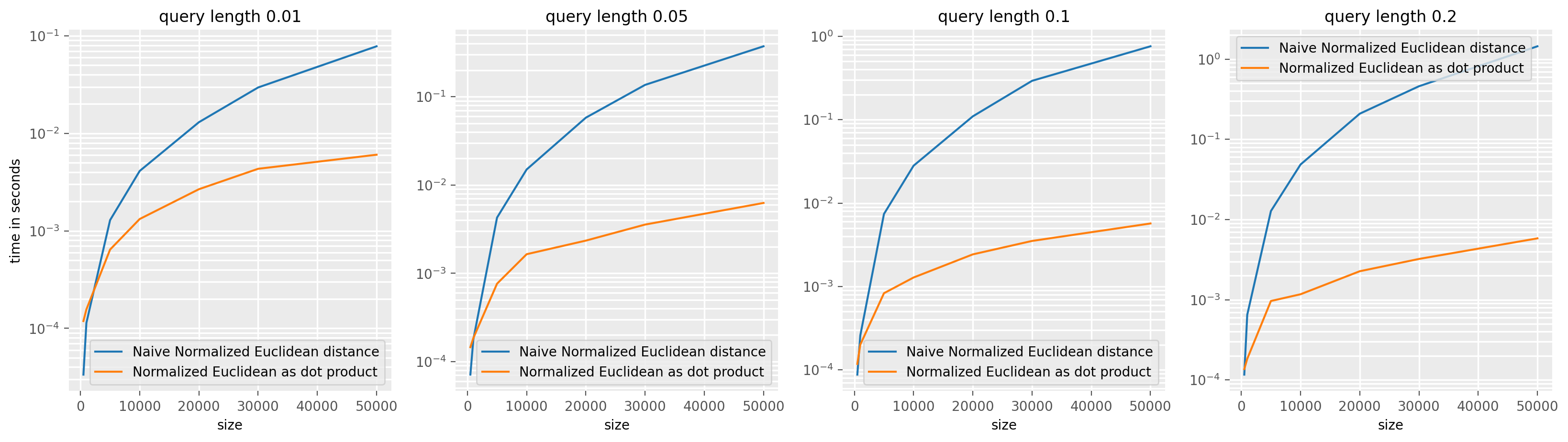
The same reasoning holds for the normalised (squared) euclidean distance, we can use the ConvolveDotProduct value for the speed_up argument in TopKSimilaritySearch to use this optimization for both normalised and non normalised distances. In the normalised case, the formula used to computed the normalised (squared) euclidean distance is taken from the paper Matrix Profile I: All Pairs Similarity Joins for Time
Series, see MASS algortihm.
[7]:
sizes = [500, 1000, 5000, 10000, 20000, 30000, 50000]
query_lengths = [0.01, 0.05, 0.1, 0.2]
times = pd.DataFrame(
    index=pd.MultiIndex(levels=[[], []], codes=[[], []], names=["size", "query_length"])
)

for size in sizes:
    for _query_length in query_lengths:
        query_length = int(_query_length * size)
        X = rng.random((1, 1, size))
        q = rng.random((1, query_length))
        n_cases, n_channels = X.shape[0], X.shape[1]
        search_space_size = size - query_length + 1
        X_means = np.zeros((n_cases, n_channels, search_space_size))
        X_stds = np.zeros((n_cases, n_channels, search_space_size))
        mask = np.ones((n_channels, search_space_size), dtype=bool)
        for i in range(X.shape[0]):
            _mean, _std = sliding_mean_std_one_series(X[i], query_length, 1)
            X_stds[i] = _std
            X_means[i] = _mean
        q_means, q_stds = sliding_mean_std_one_series(q, query_length, 1)
        q_means = q_means[:, 0]
        q_stds = q_stds[:, 0]
        # Used for numba compilation before timings
        naive_squared_distance_profile(
            X, q, mask, normalise=True, X_means=X_means, X_stds=X_stds
        )
        _times = %timeit -r 3 -n 7 -q -o naive_squared_distance_profile(X, q, mask, normalise=True, X_means=X_means, X_stds=X_stds)
        times.loc[(size, _query_length), "Naive Normalised Euclidean distance"] = (
            _times.average
        )
        # Used for numba compilation before timings
        normalised_squared_distance_profile(
            X, q, mask, X_means, X_stds, q_means, q_stds
        )
        _times = %timeit -r 3 -n 7 -q -o normalised_squared_distance_profile(X, q, mask, X_means, X_stds, q_means, q_stds)
        times.loc[(size, _query_length), "Normalised Euclidean as dot product"] = (
            _times.average
        )
[8]:
fig, ax = plt.subplots(ncols=len(query_lengths), figsize=(20, 5), dpi=200)
for j, (i, grp) in enumerate(times.groupby("query_length")):
    grp.droplevel(1).plot(label=i, ax=ax[j])
    ax[j].set_title(f"query length {i}")
    ax[j].set_yscale("log")
ax[0].set_ylabel("time in seconds")
plt.show()
Series Search
Dot products
[9]:
from aeon.similarity_search._commons import get_ith_products
from aeon.similarity_search.matrix_profiles.stomp import _update_dot_products_one_series
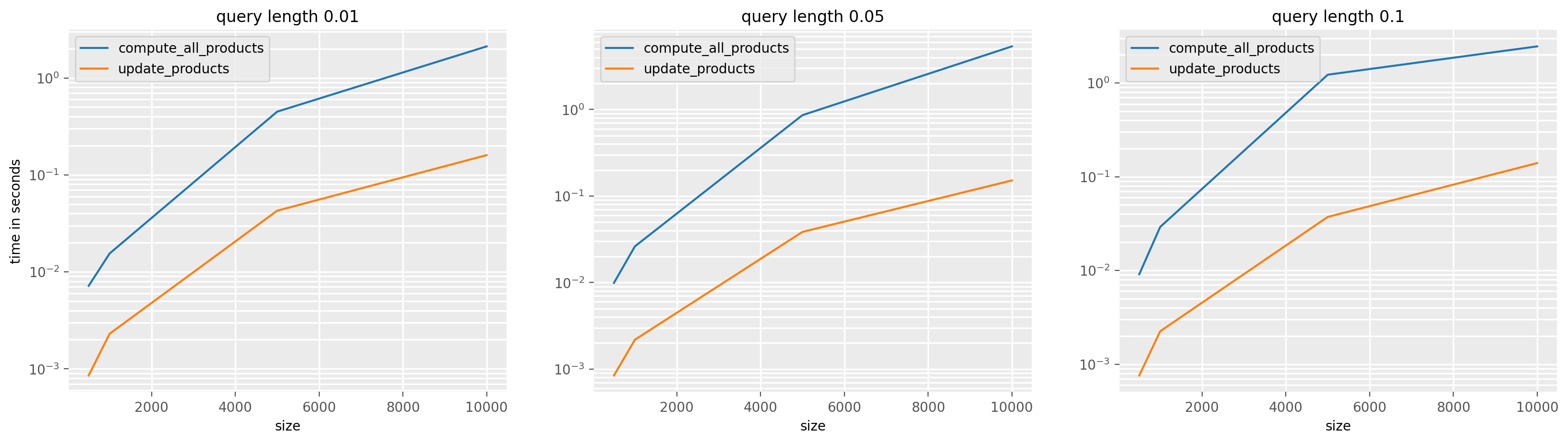
def compute_all_products(X, T, L):
"""
Compute dot products for all subsequences between two time series.
This function computes the dot products between subsequences of `X` and `T`
for a given query length `L`. It iterates over the subsequences in `T` and
calls `get_ith_products` to calculate the dot product with `X`.
"""
for i in range(T.shape[1] - L + 1):
prods = get_ith_products(X, T, L, i)
return prods
def update_products(X, T, L):
"""
Update dot products incrementally for all subsequences between two time series.
This function first computes the dot products between the first subsequence of
`X` and `T`.Then, it updates these dot products iteratively for each subsequent
subsequence in `T`.
"""
prods = get_ith_products(X, T, L, 0)
for i in range(T.shape[1] - L + 1):
prods = _update_dot_products_one_series(X, T, prods, L, i)
return prods
sizes = [500, 1000, 5000, 10000]
query_lengths = [0.01, 0.05, 0.1]
times = pd.DataFrame(
index=pd.MultiIndex(levels=[[], []], codes=[[], []], names=["size", "query_length"])
)
for size in sizes:
for _query_length in query_lengths:
query_length = int(_query_length * size)
X = rng.random((1, size))
T = rng.random((1, size))
search_space_size = size - query_length + 1
mask = np.ones((1, search_space_size), dtype=bool)
# Used for numba compilation before timings
compute_all_products(X, T, query_length)
_times = %timeit -r 3 -n 7 -q -o compute_all_products(X, T, query_length)
times.loc[(size, _query_length), "compute_all_products"] = _times.average
# Used for numba compilation before timings
update_products(X, T, query_length)
_times = %timeit -r 3 -n 7 -q -o update_products(X, T, query_length)
times.loc[(size, _query_length), "update_products"] = _times.average
[10]:
fig, ax = plt.subplots(ncols=len(query_lengths), figsize=(20, 5), dpi=200)
for j, (i, grp) in enumerate(times.groupby("query_length")):
    grp.droplevel(1).plot(label=i, ax=ax[j])
    ax[j].set_title(f"query length {i}")
    ax[j].set_yscale("log")
ax[0].set_ylabel("time in seconds")
plt.show()
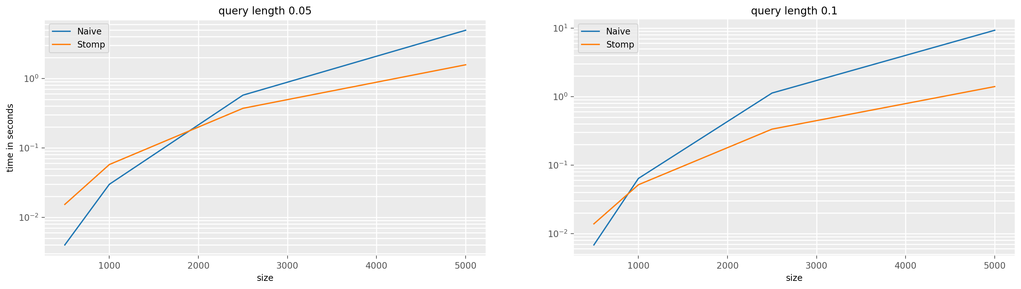
Stomp vs naive
[5]:
# Sizes are limited to not time-out the CI, you can test with more sizes locally !
sizes = [500, 1000, 2500, 5000]
query_lengths = [0.05, 0.1]
times = pd.DataFrame(
    index=pd.MultiIndex(levels=[[], []], codes=[[], []], names=["size", "query_length"])
)

for size in sizes:
    for _query_length in query_lengths:
        query_length = int(_query_length * size)
        X = rng.random((1, 1, size))
        T = rng.random((1, size))
        search_space_size = size - query_length + 1
        mask = np.ones((1, search_space_size), dtype=bool)
        # Used for numba compilation before timings
        naive_squared_matrix_profile(X, T, query_length, mask)
        _times = %timeit -r 1 -n 3 -q -o naive_squared_matrix_profile(X, T, query_length, mask)
        times.loc[(size, _query_length), "Naive"] = _times.average
        # Used for numba compilation before timings
        stomp_squared_matrix_profile(X, T, query_length, mask)
        _times = %timeit -r 1 -n 3 -q -o stomp_squared_matrix_profile(X, T, query_length, mask)
        times.loc[(size, _query_length), "Stomp"] = _times.average
[6]:
fig, ax = plt.subplots(ncols=len(query_lengths), figsize=(20, 5), dpi=200)
for j, (i, grp) in enumerate(times.groupby("query_length")):
    grp.droplevel(1).plot(label=i, ax=ax[j])
    ax[j].set_title(f"query length {i}")
    ax[j].set_yscale("log")
ax[0].set_ylabel("time in seconds")
plt.show()
[ ]:
Generated using nbsphinx. The Jupyter notebook can be found here.