Benchmarking time series regression models

Time series extrinsic regression, first properly defined in [1] then recently extended in [2], involves predicting a continuous target variable based on a time series. It differs from time series forecasting regression in that the target is not formed from a sliding window, but is some external variable.

This notebook shows you how to use aeon to get benchmarking datasets and how to compare results on these datasets with those published in [2].

Loading/Downloading data

aeon comes with two regression problems built-in the datasets module. load_covid_3month loads a univariate regression problem, while load_cardano_sentiment loads a multivariate regression problem.

from aeon.datasets import load_covid_3month

X, y = load_covid_3month()
X.shape

(201, 1, 84)

from aeon.datasets import load_cardano_sentiment

X, y = load_cardano_sentiment()
X.shape

(107, 2, 24)

The datasets used in [2] can be found in the tser_soton list in the datasets module. tser_soton_clean includes modifiers such as _eq and _nmv for datasets that were originally unequal length or had missing values. These are cleaned versions of the datasets.

from aeon.datasets.tser_datasets import tser_soton

tser_soton

['AcousticContaminationMadrid',
 'AluminiumConcentration',
 'AppliancesEnergy',
 'AustraliaRainfall',
 'BarCrawl6min',
 'BeijingIntAirportPM25Quality',
 'BeijingPM10Quality',
 'BeijingPM25Quality',
 'BenzeneConcentration',
 'BIDMC32HR',
 'BIDMC32RR',
 'BIDMC32SpO2',
 'BinanceCoinSentiment',
 'BitcoinSentiment',
 'BoronConcentration',
 'CalciumConcentration',
 'CardanoSentiment',
 'ChilledWaterPredictor',
 'CopperConcentration',
 'Covid19Andalusia',
 'Covid3Month',
 'DailyOilGasPrices',
 'DailyTemperatureLatitude',
 'DhakaHourlyAirQuality',
 'ElectricityPredictor',
 'ElectricMotorTemperature',
 'EthereumSentiment',
 'FloodModeling1',
 'FloodModeling2',
 'FloodModeling3',
 'GasSensorArrayAcetone',
 'GasSensorArrayEthanol',
 'HotwaterPredictor',
 'HouseholdPowerConsumption1',
 'HouseholdPowerConsumption2',
 'IEEEPPG',
 'IronConcentration',
 'LiveFuelMoistureContent',
 'LPGasMonitoringHomeActivity',
 'MadridPM10Quality',
 'MagnesiumConcentration',
 'ManganeseConcentration',
 'MethaneMonitoringHomeActivity',
 'MetroInterstateTrafficVolume',
 'NaturalGasPricesSentiment',
 'NewsHeadlineSentiment',
 'NewsTitleSentiment',
 'OccupancyDetectionLight',
 'ParkingBirmingham',
 'PhosphorusConcentration',
 'PotassiumConcentration',
 'PPGDalia',
 'PrecipitationAndalusia',
 'SierraNevadaMountainsSnow',
 'SodiumConcentration',
 'SolarRadiationAndalusia',
 'SteamPredictor',
 'SulphurConcentration',
 'TetuanEnergyConsumption',
 'VentilatorPressure',
 'WaveDataTension',
 'WindTurbinePower',
 'ZincConcentration']

You can download and load these problems from .ts files with the load_regression function. load_from_ts_file is also available if you want to load from file.

from aeon.datasets import load_regression

X_train_bc, y_train_bc = load_regression("BarCrawl6min", split="train")
X_test_bc, y_test_bc = load_regression("BarCrawl6min", split="test")
(X_train_bc.shape, y_train_bc.shape), (X_test_bc.shape, y_test_bc.shape)

(((140, 3, 360), (140,)), ((61, 3, 360), (61,)))

Evaluating a regressor on benchmark data

With the data, it is easy to assess an algorithm performance. We will use the DummyRegressor as a baseline which takes the mean of the target, and use R2 score as our scoring metric.

This should be familiar to anyone who has used scikit-learn before.

from sklearn.metrics import r2_score

from aeon.regression import DummyRegressor

small_problems = [
    "BarCrawl6min",
    "CardanoSentiment",
    "Covid3Month",
    "ParkingBirmingham",
    "FloodModeling1",
]

dummy = DummyRegressor()
performance = []
for problem in small_problems:
    X_train, y_train = load_regression(problem, split="train")
    X_test, y_test = load_regression(problem, split="test")

    dummy.fit(X_train, y_train)
    pred = dummy.predict(X_test)

    mse = r2_score(y_test, pred)
    performance.append(mse)

    print(f"{problem}: {mse}")

BarCrawl6min: -0.012403529243674827
CardanoSentiment: -0.21576890538877036
Covid3Month: -0.004303695576216793
ParkingBirmingham: -0.0036438945855674643
FloodModeling1: -0.0016071827276951112

Comparing to reference/published results

How do the dummy results compare to the published results in [2]? We can use the get_estimator_results and get_estimator_results_as_array methods to load published results.

get_available_estimators will show you the available estimators with stored results the task.

from aeon.benchmarking.results_loaders import get_available_estimators

get_available_estimators(task="regression")

	regression
0	1NN-DTW
1	1NN-ED
2	5NN-DTW
3	5NN-ED
4	CNN
5	DrCIF
6	FCN
7	FPCR
8	FPCR-b-spline
9	FreshPRINCE
10	GridSVR
11	InceptionTime
12	RandF
13	ResNet
14	Ridge
15	ROCKET
16	RotF
17	SingleInceptionTime
18	XGBoost

get_estimator_results will load the results to a dictionary of dictionaries with regressors and datasets as the keys. ParkingBirmingham was originally unequal length, so we remove the _eq from the end of the results key to match the dataset name using a parameter.

from aeon.benchmarking.results_loaders import get_estimator_results

regressors = ["DrCIF", "FreshPRINCE"]
results_dict = get_estimator_results(
    estimators=regressors,
    datasets=small_problems,
    num_resamples=1,
    task="regression",
    measure="r2",
    remove_dataset_modifiers=True,
)
results_dict

{'DrCIF': {'BarCrawl6min': 0.44579994072037,
  'CardanoSentiment': -0.3243974127240141,
  'Covid3Month': 0.0710586822956002,
  'ParkingBirmingham': 0.7139985894810016,
  'FloodModeling1': 0.8965591366052275},
 'FreshPRINCE': {'BarCrawl6min': 0.3936563948097531,
  'CardanoSentiment': -0.1300226564057678,
  'Covid3Month': 0.1888015511133555,
  'ParkingBirmingham': 0.7304688812606739,
  'FloodModeling1': 0.9296442893073922}}

get_estimator_results will instead load an array. Note that if multiple resamples are loaded, the results will be averaged using this function.

from aeon.benchmarking.results_loaders import get_estimator_results_as_array

results_arr, names = get_estimator_results_as_array(
    estimators=regressors,
    datasets=small_problems,
    num_resamples=1,
    task="regression",
    measure="r2",
    remove_dataset_modifiers=True,
)
results_arr

array([[ 0.44579994,  0.39365639],
       [-0.32439741, -0.13002266],
       [ 0.07105868,  0.18880155],
       [ 0.71399859,  0.73046888],
       [ 0.89655914,  0.92964429]])

The names of the datasets are also returned as missing values are removed from the results by default. Each row corresponds to a dataset and each column to a regressor.

names

['BarCrawl6min',
 'CardanoSentiment',
 'Covid3Month',
 'ParkingBirmingham',
 'FloodModeling1']

we just need to align our results from the website so they are aligned with the results from our dummy regressor

Do the same for our dummy regressor results

import numpy as np

regressors = ["DrCIF", "FreshPRINCE", "Dummy"]
results = np.concatenate([results_arr, np.array(performance)[:, np.newaxis]], axis=1)
results

array([[ 0.44579994,  0.39365639, -0.01240353],
       [-0.32439741, -0.13002266, -0.21576891],
       [ 0.07105868,  0.18880155, -0.0043037 ],
       [ 0.71399859,  0.73046888, -0.00364389],
       [ 0.89655914,  0.92964429, -0.00160718]])

Comparing Regressors

aeon provides visualisation tools to compare regressors.

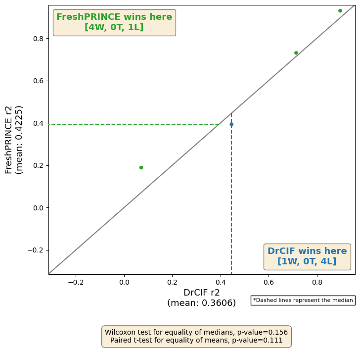
We can plot the results against each other. This also presents the wins and losses and some summary statistics.

from aeon.visualisation import plot_pairwise_scatter

plot_pairwise_scatter(
    results[:, 0],
    results[:, 1],
    "DrCIF",
    "FreshPRINCE",
    metric="r2",
)

(<Figure size 800x800 with 1 Axes>,
 <Axes: xlabel='DrCIF r2\n(mean: 0.3606)', ylabel='FreshPRINCE r2\n(mean: 0.4225)'>)

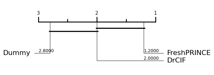
We can plot the results of multiple regressors on a critical difference diagram [3], which shows the average rank and groups estimators by whether they are significantly different from each other.

from aeon.visualisation import plot_critical_difference

plot_critical_difference(results, regressors)

(<Figure size 600x220 with 1 Axes>, <Axes: >)

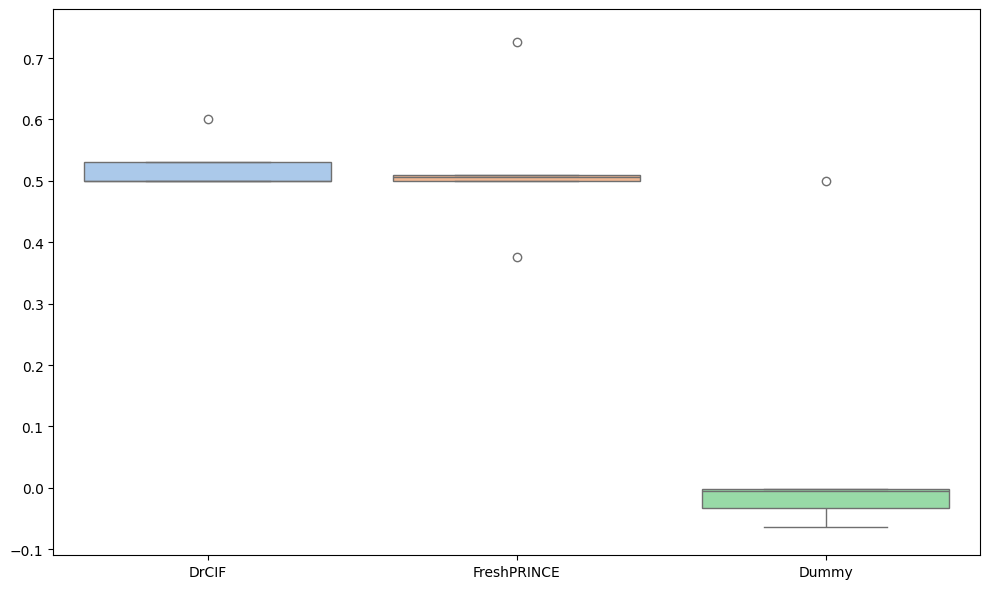
A function for plotting a boxplot is also available.

from aeon.visualisation import plot_boxplot

plot_boxplot(results, regressors, relative=True, plot_type="boxplot")

(<Figure size 1000x600 with 1 Axes>, <Axes: >)

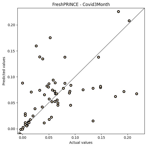
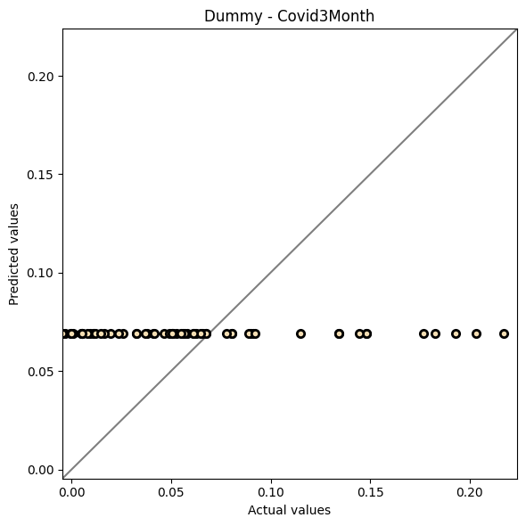
Sometimes it is interesting to compare the performance of estimators on a single specific dataset. We use the BarCrawl6min dataset here.

from aeon.regression import DummyRegressor
from aeon.regression.feature_based import FreshPRINCERegressor

fp = FreshPRINCERegressor(n_estimators=10, default_fc_parameters="minimal")
fp.fit(X_train_bc, y_train_bc)
y_pred_fp = fp.predict(X_test_bc)

d = DummyRegressor()
d.fit(X_train_bc, y_train_bc)
y_pred_d = d.predict(X_test_bc)

from aeon.visualisation import plot_scatter_predictions

plot_scatter_predictions(y_test_bc, y_pred_fp, title="FreshPRINCE - Covid3Month")

(<Figure size 600x600 with 1 Axes>,
 <Axes: title={'center': 'FreshPRINCE - Covid3Month'}, xlabel='Actual values', ylabel='Predicted values'>)

plot_scatter_predictions(y_test_bc, y_pred_d, title="Dummy - Covid3Month")

(<Figure size 600x600 with 1 Axes>,
 <Axes: title={'center': 'Dummy - Covid3Month'}, xlabel='Actual values', ylabel='Predicted values'>)

References

[1] Tan, C.W., Bergmeir, C., Petitjean, F. and Webb, G.I., 2021. Time series extrinsic regression: Predicting numeric values from time series data. Data Mining and Knowledge Discovery, 35(3), pp.1032-1060.

[2] Guijo-Rubio, D., Middlehurst, M., Arcencio, G., Silva, D.F. and Bagnall, A., 2024. Unsupervised feature based algorithms for time series extrinsic regression. Data Mining and Knowledge Discovery, pp.1-45.

[3] Garcia, S. and Herrera, F., 2008. An Extension on” Statistical Comparisons of Classifiers over Multiple Data Sets” for all Pairwise Comparisons. Journal of machine learning research, 9(12).

---

Generated using nbsphinx. The Jupyter notebook can be found here.